
ChatGPT Doesn’t Think. It Pays Attention.
A plain-English tour of Transformers, GPT, and LLMs (with just enough math)

Image Source: XKCD
Reading guide: This is a long post (~40 min read). Here is how to navigate it.
Want the full picture? Read straight through. Each section builds on the last.
Already know what RNNs are? Skip to Act 2: The Transformer.
Just want to understand GPT/ChatGPT? Jump to Act 3: From Transformer to GPT.
Curious about scaling, RLHF, or reasoning? Head to Act 4: From GPT to LLMs.
Short on time? Read the recap in Act 5 for the full story in a few paragraphs.

Act 1: Introduction
You’ve probably used ChatGPT today. Or maybe Google Translate, or Gemini, Claude, or one of the dozen AI tools that have quietly crept into our everyday life over the past couple of years. Typically, you type something in (or talk) and the AI just… it just responds. It feels like magic, or at least like something impossibly complex (in my opinion, it is, lol).
Personally, I started dabbling with ChatGPT back in 2023 while working on my senior thesis in college. I was building a machine learning system to detect security bugs in C/C++ code. Throughout all my prompting, I had this nagging feeling that everything I was doing was almost useless, because I knew I could give ChatGPT the code and it would find those bugs itself. Or it could be fine-tuned to do so, similar to how Wiz, the cybersecurity startup, did to a Llama model. It is such powerful technology.

The interesting thing, however, is that all these tools, every single one of them, run on the same core idea; an idea from a single paper published in 2017 by a team of researchers at Google. The paper is called “Attention Is All You Need”, and it introduced the Transformer. If you’ve heard the term and wondered what it actually means, or if you’ve never heard it and want to understand what’s going on when you talk to ChatGPT, this post is for you.
This is the first post in a two-part series. We’ll cover Transformers and LLMs here, then tackle agents and coding tools (like Claude Code) in upcoming posts. We’ll also touch briefly on the “thinking” part of LLMs (reasoning). That said, for now we’ll focus just on text, not images, audio, or other modalities, even though those are mostly built on the same underlying tech.
Let’s get into it.
The World Before Transformers
Image Source: oxen.ai
Before we can appreciate what the Transformer did, we need to understand what existed before it.
Before 2017, the dominant approach for language tasks (translation, text generation, etc.) was the Recurrent Neural Network (RNN) and its more popular variants LSTMs (Long Short-Term Memory) and GRUs (Gated Recurrent Units). The straightforward idea at the core of these models was to process text sequentially, one word at a time, from left to right, and at each step update an internal “memory” (called a hidden state) that tries to capture everything the model has read so far.
You can think of it like reading a book through a mail slot (or using one of those speed reader apps that use Rapid Serial Visual Presentation (RSVP). You see one word, you try to remember it, then the next word comes, and you try to fold that into what you already remember. However, by the time you’re 50 words in, your memory of word 1 is fuzzy at best (even if you might have a rough idea of what you read). The hidden state in RNNs is a fixed-size vector that tries to compress an ever-growing amount of information, and eventually, something has to give.
Using these models created two big problems:
They are slow. (Unlike speed reading with RSVP). Because RNNs process words sequentially (word 1 must be processed before word 2, word 2 before word 3, and so on), you can’t parallelize the computation. Each step depends on the previous one. This made training painfully slow, especially on longer sequences. As GPUs got faster at handling many tasks simultaneously, RNNs couldn’t take advantage of that because their architecture was fundamentally sequential.
They were forgetful. That fixed-size hidden state was a bottleneck. Long-range dependencies (where a word early in a sentence is crucial for understanding a word much later) are hard for the model to learn. Consider the sentence: “The cat that chased the dog that barked at the mailman sat on the mat.” By the time the model reaches “sat,” the hidden state’s memory of “cat” (the actual subject) has been diluted by everything in between. This is related to what’s known as the vanishing gradient problem: as the model learns connections over long distances, the training signal becomes weaker and weaker. Like a game of telephone, the final state has limited context on the initial states.
Researchers knew this was a problem, and they tried to fix it. LSTMs and GRUs were specifically designed to be better at retaining information across longer sequences, and they helped, but they didn’t solve the fundamental bottleneck. The hidden state remained a fixed-size summary of everything that had come before.
Then, in 2014, we had a breakthrough. Attention mechanisms (introduced by Bahdanau et al.) gave models the ability to “look back” at any part of the input when generating each word of the output, instead of relying entirely on that compressed hidden state. This was a huge improvement for tasks like translation. But attention was still being used in addition to the RNN, not instead of it. Hence, the sequential processing bottleneck still existed.
Then came the 2017 paper that changed everything. A group of researchers at Google experimented with a simple, but honestly, radical idea: what if we got rid of recurrence entirely and relied only on attention?
The result was the Transformer. And it worked so well that it became the default backbone for modern language models.
Act 2: The Transformer
Thus far, we have identified the problem: RNNs process words one at a time and struggle with long-range dependencies. We have also established that the solution is the Transformer, which relies on Attention. But what is Attention? Let’s build up our understanding using three analogies.
The Cocktail Party
Imagine you’re at a crowded party. There are dozens of conversations happening around you all at once. Music is playing, people are laughing, some people are dancing, others are drinking. Despite all the noise, when someone across the room says your name, your brain instantly locks onto that signal. You didn’t need to listen to every conversation in sequence to find the relevant one. Your brain, in a sense, just attended (or paid attention) to the right thing.
You can also split your focus. You might be talking to someone, but part of your brain is monitoring an interesting conversation happening nearby. You’re processing multiple streams of information in parallel, dynamically deciding what’s relevant and what to ignore.
That’s the core intuition behind attention in machine learning. Instead of processing information one piece at a time and hoping a hidden state remembers what matters, what if the model could “hear” the entire input at once and dynamically focus on the most relevant parts? In a Transformer, “locking on” means assigning larger numerical weights to certain tokens and smaller weights to others.
That is what the Transformer does. But “dynamically focus” is still vague, so we have to get more concrete.
The Library
Say you walk into a library with a specific research question. For instance, “What was the world like when the dinosaurs were alive?” That question is your Query or what you are looking for.
Every book on the shelf has a title and a short description on its spine. Those are the Keys, letting you know what each book is about.
Now, you scan the shelves. Your brain automatically scores how relevant each book is to your research question. A book about exactly your topic (in our case, that could be The Complete Book of Dinosaurs) would have high relevance. A book about something tangentially related, for instance, Asteroids: Astronomical and Geological Bodies, would have low relevance. And a book about something completely unrelated (let’s say a book about how Toy Story was animated) would have basically near-zero relevance.
Now, here’s where things get interesting. Instead of just grabbing the single most relevant book, you pull information from many books, each one contributing in proportion to how relevant it was to your question. These contributions are the Values, the actual content each book offers. A highly relevant book significantly enhances your understanding. A barely relevant one contributes almost nothing, but isn’t completely ignored either.
The result is a weighted combination of information from across the entire library, tailored specifically to your question. That’s attention, or a blending of all available information, weighted by relevance.
The Google Search
Now that we have the intuition from the library, let’s map it to something even more familiar and then jump straight into the math.
You type a search query into Google (or Bing — yes, people use Bing). That’s your Q. Google compares that query against the titles and descriptions of billions of pages (the Ks), scores each page’s relevance, and returns results weighted by those scores. The actual content of each page (the Vs) gets weighted by relevance, so the top results get your attention, while page-ten results barely register. One difference worth noting, though, is that Google shows you a ranked list of separate results, whereas Attention blends all the results into a single, relevance-weighted output.
The mapping here is actually clean enough that we can walk through the actual math. Here’s the equation from the paper:
If that looks intimidating, don’t worry; we’ll break it down piece by piece. But first, let’s establish some building blocks so we know what Q, K, and V actually are.
The Building Blocks
Q, K, and V are not words themselves; they’re vectors (lists of numbers) derived from the input tokens. For every token, the model creates three different vector “versions”: a Query (“what am I looking for?”), a Key (“how should others find me?”), and a Value (“what information do I contribute?”). So if your sentence has 10 tokens, you have 10 query vectors (one per token), stacked into the matrix Q. Same for K and V. Attention uses Query–Key matching to figure out what’s relevant, then uses those relevance scores to blend the Values.
But where do these vectors come from? Let’s trace the path from raw text to math.
Tokens
Models don’t operate on whole words. They operate on tokens, which are word pieces.
For example, “unbelievable” might become tokens like: [“un”, “believ”, “able”]
Each token has a unique numerical identifier.
So your sentence:
“The cat sat.”
might become tokens: [“The”, “cat”, “sat”] that map to token IDs: [713, 4583, 987]
Embeddings
Now we need to convert those IDs into a form the model can work with mathematically. That’s where embeddings come in.
An embedding is a learned lookup table in which each token ID maps to a vector (a list of numbers). At first, these vectors are random. During training, they get adjusted so that tokens used in similar contexts end up with vectors that are close together.
In practice, the Transformer has an embedding table with one row per token in its vocabulary (e.g., 50,000 rows) and a fixed number of columns (e.g., 768). Looking up an embedding is simple:
embedding_table[token_id] = vector of numbers
So if the token ID for “cat” is 4583, you look up row 4583 and get its embedding vector:
cat -> [0.12, -1.80, 0.03, 2.10, ...]
In real models, these vectors are typically hundreds or thousands of numbers long (e.g., 512, 768, 4096). The key idea is that similar words tend to have similar vectors. For instance, “king” and “queen” would be close together, while “king” and “toaster” would be far apart.
Position Information
There’s one more thing we need before we can feed tokens into the attention module. If we only used embeddings, these two inputs would look identical (same tokens, same embeddings):
“cat sat on mat”
“mat on sat cat”
Word order matters, so we add positional encoding as a way of “tagging” each token with where it appears in the sentence. In simple terms, every token’s embedding gets a small numerical adjustment based on its position. We’ll explore exactly how this works later in this post, but for now, know that after this step, each token has a vector that captures both what the token means and where it appears.
The result is that each token in your input is now represented as a vector that encodes meaning and position. These are the vectors that get transformed into Q, K, and V for the attention mechanism.
Here’s the full pipeline:
Text → Tokens → Token IDs → Embedding Vectors → Add Position → Token Vectors (ready for attention)
Now let’s break down the attention equation.
The Attention Equation, Step by Step
One important note before we begin: if your sentence has n tokens, then Q and K are each like tables with n rows (one row per token) and d_k columns. When we compute QKᵀ, the result is an n × n table of every token scored against every other token. It’s a grid of “who cares about whom.”
Step 1: Score how relevant each key is to your query.
When you Google something, the search engine needs to figure out which pages are relevant to what you typed. Mathematically, one way to measure how similar two things are is the dot product. If two vectors point in the same direction, their dot product is high; if they’re unrelated, it’s low. So we take the dot product of the Query with every Key:
Each score indicates how well a particular key matches the given query. We use the transpose of K (Kᵀ) so that the matrix dimensions line up correctly for the dot product. Q has shape (n × d_k), and Kᵀ has shape (d_k × n), giving us that (n × n) table of scores.
Step 2: Scale the scores down.
Here’s a practical problem. When the vectors are high-dimensional (as in Transformers), dot products can be very large in magnitude. Large values push the softmax function (next step) into extreme territory where one score could dominate, and everything else gets crushed to near-zero. So we divide by √d_k (the square root of the key dimension) to keep things in a reasonable range. You can think of this as volume control. We’re turning down the loudest values so the quieter ones don’t get drowned out.
Step 3: Convert scores to weights.
Right now, we have raw scores; some large, some small, some negative. We need to turn these into clean proportions that add up to 1, so we can use them as weights. That’s what the softmax function does. It takes any set of numbers and squishes them into a probability distribution: the biggest score gets the biggest weight, smaller scores get smaller weights, and everything sums to 1.
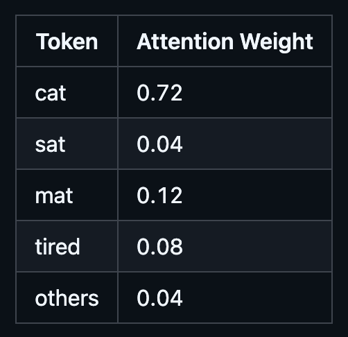
To make this concrete, let’s go back to our sentence: “The cat sat on the mat because it was tired.”
When computing attention for the token “it,” the model might assign weights like:
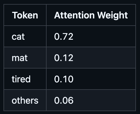
The model has figured out that “it” most likely refers to “cat”, so “cat” gets the lion’s share of the attention.
Step 4: Use the weights to blend the values.
Now we have a weight for every token in the input. The final step is to multiply each Value by its weight and add them all up:
The result isn’t a single vector for the whole sentence, but rather an output vector per token. Each token gets its own context-aware version of itself, updated using information from the tokens it attended to. The token “it” now carries information that’s heavily influenced by “cat,” because that’s what the attention weights determined was most relevant.
This gives us the full equation:
Hence, we have the four steps written as one expression. Score, scale, normalize, blend.
If you want to see what it looks like in code, here’s a simplified version in Python using numpy:
import numpy as np

def attention(Q, K, V):
    d_k = K.shape[-1]
    scores = Q @ K.T                # Step 1: dot product (relevance scores)
    scores = scores / np.sqrt(d_k)  # Step 2: scale down
    weights = softmax(scores)       # Step 3: convert to weights (0 to 1, sum to 1)
    output = weights @ V            # Step 4: weighted blend of values
    return output
These four steps are deceptively simple when laid out like this, but arriving at this formula took years of research, failed experiments, and the combined effort of dozens of researchers building on each other’s work. The simplicity of the final result is a testament to how much hard work it took to get there. Now let’s see what happens when you put it to work.
Self-Attention: Every Word Queries Every Other Word
Here is where things get clever. In the library analogy, we imagined one researcher walking in with one question. But in a Transformer, every word in the input is the researcher. Every single token forms its own Query and asks, “What in this sentence is relevant to me?” At the same time, every token offers up its Key and its Value to all the other tokens. And all of this happens simultaneously, in parallel, for every token in the input.
This is called self-attention (sometimes called intra-attention), and it is the mechanism that makes Transformers tick. The “self” part means that the Queries, Keys, and Values all come from the same sequence. The model is not looking at some external source of information. It is looking at itself, figuring out the internal relationships between its own tokens.
Let’s walk through what this looks like with a concrete example. Take this sentence:
“The cat sat on the mat because it was tired.”
When the model is processing the token “it,” it needs to figure out what “it” refers to. Is it the cat? The mat? Something else? With self-attention, the token “it” produces a Query vector. Every other token produces a Key vector. The model compares the Query for “it” against all of these Keys using dot products, and the score between “it” and “cat” ends up being high because the model has learned representations where these tokens are closely related in this context. The score with “mat” is lower. Similarly with “the” or “on.”
After softmax, the attention weights might look something like this:
So the output vector for “it” becomes heavily influenced by the Value vector of “cat.” In plain English, the model has updated the representation of “it” to carry information from “cat.” This resembles what linguists call coreference resolution, the problem of determining what a pronoun refers to in a text. The remarkable thing is that Transformers often learn to do this kind of behavior implicitly, just from training on large amounts of text.
And here is the part that matters most for performance. Remember how RNNs had to pass information step by step through the hidden state? If “cat” is 10 words away from “it,” the RNN needs 10 sequential steps (with 10 chances to lose information along the way) to connect them. With self-attention, the path length between any two tokens is O(1), meaning constant. It does not matter if the two words are next to each other or 500 tokens apart. The attention mechanism connects them directly in a single step. This is one of the key advantages highlighted in Table 1 of the original paper, where self-attention achieves O(1) maximum path length compared to O(n) for recurrent layers. To understand more about the notation, you can read about Big-O here.
The tradeoff is computational cost. That n × n attention matrix means self-attention scales quadratically with sequence length (O(n² · d) per layer). For short and medium sequences, this is fine, and the parallelism more than makes up for it. For very long sequences (tens of thousands of tokens), this becomes expensive, which is a big part of why running LLMs costs so much. There is a large and ongoing research effort to make attention more efficient. A good overview is this survey on efficient Transformers, and implementations like FlashAttention have made significant progress on the practical side by optimizing how attention runs on GPUs. But for the original Transformer and most models you interact with today, the full n × n attention is what runs under the hood.
One last thing before we move on. Self-attention by itself has no built-in notion of word order. The attention scores are computed purely from the content of the vectors, not from where they appear in the sentence. That is exactly why we added positional encodings back in the building blocks section. Without them, “The cat sat on the mat” and “mat the on sat cat the” would produce identical attention patterns. Positional encodings give the model the ordering information it needs so that attention can focus on what matters while still knowing where everything is.
Multi-Head Attention: More Than One Perspective

So we have self-attention. Every token can attend to every other token and produce a context-aware output. That is powerful on its own. But there is a problem.
A single attention head computes one set of attention weights. That means each token gets one “opinion” about what is relevant. But language is complicated. When you read a sentence, multiple things are going on at the same time. Consider:
“The cat sat on the mat because it was tired.”
To fully understand this sentence, you need to track several different kinds of relationships simultaneously:
Grammar: “cat” is the subject, “sat” is the verb; they need to agree.
Reference: “it” refers to “cat,” not “mat.”
Proximity: “on” relates to “mat” (what it sat on) and “sat” (the action).
A single attention head must represent all these different relationships using a single attention pattern. That is a lot to ask. It is like asking one person to read a sentence, track its grammar, meaning, and structure, and report back with a single answer. The original paper describes this limitation as “averaging inhibits” the model’s ability to attend to information from different representation subspaces.
As you can tell, that would be challenging. So the solution is to ask several people rather than just one.
How It Works
Multi-head attention runs multiple attention functions in parallel, each one independently learning to focus on a different type of relationship. The original Transformer paper uses 8 heads (so 8 parallel attention functions), but other models use different numbers (12, 16, 32, etc.).
Here is how it works step by step:
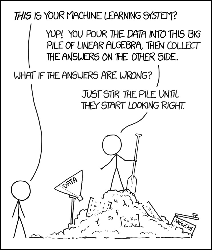
Image Source: XKCD
Project into smaller spaces. For each head, the model takes the input vectors and projects them into a smaller set of Q, K, and V vectors using learned linear transformations (basically learned weight matrices). If the model dimension is 512 and there are 8 heads, each head works with vectors of size 512 / 8 = 64. This is where the Q, K, and V vectors actually get created. Each head learns its own set of projection weights, which means each head learns to “look at” the input differently.
Run attention independently. Each head takes its own Q, K, and V and runs the same attention calculation we covered earlier (dot product, scale, softmax, blend) and produces its own output.
Concatenate and project back. The outputs from all 8 heads are concatenated (stuck together side by side) into a single long vector. Then a final linear transformation projects it back to the original model dimension.
In equation form:
where each head is:
The Wᵢ_Q, Wᵢ_K, and Wᵢ_V are the learned projection matrices for head i. They are what allow each head to develop its own “perspective” on the input. Wᴼ is the final output projection that combines everything back together.
Here is a simplified code version (note that real implementations are more efficient, projecting once and reshaping rather than looping, but this captures the logic clearly):
def multi_head_attention(Q, K, V, W_q, W_k, W_v, W_o, num_heads):
    heads = []
    for i in range(num_heads):
        Q_i = Q @ W_q[i]           # project Q for this head
        K_i = K @ W_k[i]           # project K for this head
        V_i = V @ W_v[i]           # project V for this head
        head_i = attention(Q_i, K_i, V_i)  # run attention
        heads.append(head_i)

    concatenated = concat(heads)   # stick all outputs together
    output = concatenated @ W_o    # project back to model dimension
    return output
What the Heads Actually Learn
The key insight is that because each head has its own learned projections, different heads end up specializing in different things. The model is not told what to specialize in. This happens naturally during training.
The attention visualizations in the original paper (Figures 3, 4, and 5) show this clearly. For the sentence “The Law will never be perfect, but its application should be just,” different heads in layer 5 learned very different behaviors:
One head learned to connect “its” to “Law” (resolving what “its” refers to).
Another head learned to track the overall syntactic structure of the sentence.
Yet another seemed to focus on adjacent word relationships.
Nobody programmed these behaviors. The heads figured them out on their own because having multiple specialized perspectives is much more effective than having one general-purpose perspective. Jay Alammar’s illustrated guide has great visualizations of this if you want to see more examples.
Why Not Just Use a Bigger Single Head?
You might wonder why we don’t just make one attention head bigger instead of using 8 smaller ones. The paper actually tested this (see Table 3, rows (A)). Single-head attention performed about 0.9 BLEU (Bilingual Evaluation Understudy), which measures the quality of generated text, points worse than the best multi-head configuration, even when the total computation was kept the same. Interestingly, too many heads also hurt performance. 8 heads turned out to be a sweet spot for their model.
The reason multi-head works better is that a single head, no matter how big, produces a single set of attention weights. It has to average across all the different types of relationships. Multi-head attention avoids this by giving each head the freedom to specialize, and then combining their outputs. It is like the difference between asking one generalist and asking a team of specialists.
A Note on Cost
You might worry that running 8 attention functions is 8 times more expensive. It is not. Because each head operates on vectors of dimension d_model / h (64 instead of 512 in the base model), the total computational cost is roughly the same as running a single attention head with the full dimension. You get the benefit of multiple perspectives without paying extra. This is pointed out in Section 3.2.2 of the original paper.
Positional Encoding: Teaching the Model Word Order
We touched on this briefly in the building blocks section, but it warrants a closer look.
Here is the problem again. Self-attention computes scores based purely on the content of the vectors. It does not care where a token appears in the sequence. Without any positional information, the model would have no way to tell apart “the cat chased the dog” and “the dog chased the cat.” They contain the same tokens, so as far as attention is concerned, they look identical. Obviously, those sentences mean very different things.
RNNs did not have this problem because they processed tokens in order. Position was baked into the architecture. But the Transformer threw out sequential processing in favor of parallelism, so it needs another way to know where things are.
The solution is to add a positional encoding to each token’s embedding before feeding it into the model. The positional encoding is a vector of the same size as the embedding, and you simply add them together element by element:
where X is the token embedding and P is the positional encoding. If your sequence has n tokens, then X is an n × d_model table of embeddings and P is an n × d_model table of positional encodings. You add them row by row, so each token’s vector ends up carrying information about both what the token is and where it appears.
How the Original Paper Does It
The authors of “Attention Is All You Need” used sine and cosine functions at different frequencies to generate positional encodings. The formulas are:
where pos is the position in the sequence (0, 1, 2, …) and i is the dimension index.
You do not need to memorize these formulas. The only thing that matters is that every position gets a unique pattern of numbers.
That said, the intuition behind them is actually straightforward. Think of it like an odometer in a car. The rightmost digit changes fastest (every mile), the next digit changes every 10 miles, the next every 100 miles, and so on. Each “digit” cycles at a different rate, so every mileage reading is unique.
Sinusoidal positional encodings work the same way. Each dimension of the encoding oscillates at a different frequency. The early dimensions cycle quickly (changing significantly between adjacent positions), while the later dimensions cycle slowly (changing gradually over long stretches of the sequence). The combination of all these frequencies at different rates gives every position a unique “fingerprint.”
This design has a nice property: for any fixed k distance between two positions, the positional encoding of pos + k can be expressed as a linear function of the encoding at pos. This means the model can potentially learn to attend by relative position (how far apart two tokens are) rather than just absolute position (what position number each one has).
Do You Have to Use Sinusoids?
No. The paper also experimented with learned positional embeddings (where the model learns a separate vector for each position during training, similar to how it learns token embeddings) and found that both approaches produced nearly identical results (see Table 3, row (E)).
The authors chose sinusoidal encodings because they hypothesized that it would allow the model to generalize to sequence lengths longer than anything it saw during training. Since the sine and cosine functions are defined for any position, the model does not encounter the “I’ve never seen position 5001” problem that a learned embedding table would.
In practice, many modern Transformer models use entirely different approaches. For instance, Rotary Position Embeddings (RoPE) have become popular in recent LLMs because they encode relative position directly into the attention computation. But the core idea remains the same: the model needs some way to know where tokens are, and positional encodings provide that.
Putting It All Together: The Full Transformer Architecture
We now have all the pieces. Let’s see how they fit together.
The Transformer follows an encoder-decoder structure, which was common in sequence-to-sequence models before it. The encoder reads the input (for example, a French sentence) and builds a rich representation of it. The decoder takes that representation and generates the output (the English translation) one token at a time.
What makes the Transformer different is how the encoder and decoder are built. Instead of recurrent layers, they are built entirely from the components we’re learning about in this post.
Let’s walk through each part.
The Encoder
The encoder is a stack of N = 6 identical layers (in the base model). Each layer has two sub-layers:
Multi-head self-attention. Every token in the input attends to every other token, exactly as we described. This is where the model builds context-aware representations.
A position-wise feed-forward network. After attention gathers information from across the sequence, this network processes each token independently. It consists of two linear transformations with a ReLU activation in between:
\(\text{FFN}(x) = \max(0,\ xW_1 + b_1)W_2 + b_2\)
You can think of the division of labor this way: attention figures out what information to gather from other tokens, and the feed-forward network figures out what to do with that gathered information. The feed-forward network applies the same transformation to each token position independently, but it uses different learned parameters at each layer. In the base model, the input and output dimensions are d_model = 512, and the inner layer has a dimension of d_ff = 2048.
Each of these two sub-layers also has two additional components wrapped around it:
Residual connections. The output of each sub-layer is added back to its input before moving on. In other words, the model computes x + SubLayer(x) rather than just SubLayer(x). This idea comes from deep residual networks (ResNets), and it solves a practical problem: in deep networks (with many layers), information can get lost or distorted as it passes through layer after layer. By adding the input back to the output, the model always has access to the original information. If a layer does not learn anything useful, the residual connection lets the signal pass through unchanged rather than getting corrupted. Think of it like keeping a photocopy of a document before editing it. If the edits make things worse, you still have the original.
Layer normalization. After each residual connection, the model normalizes the values to keep them in a stable range. Without normalization, the numbers flowing through the network can gradually grow very large or very small as they pass through layer after layer, making training unstable. Layer norm keeps things well-behaved.
So the full operation for each sub-layer is:
Stack 6 of these layers on top of each other, and that is the encoder. The input tokens go in at the bottom (after embedding and positional encoding), flow through all 6 layers, and what comes out at the top is a set of context-aware representations, one per token, that capture the meaning of the entire input sequence.
The Decoder
The decoder is also a stack of N = 6 identical layers, but each layer has three sub-layers instead of two:
Masked multi-head self-attention. This is the same self-attention as in the encoder, with one crucial difference: masking. When the model is generating output, it produces tokens one at a time, left to right. When predicting token 5, it should only see tokens 1 through 4. It must not be able to peek at tokens 6, 7, 8, and beyond, because those have not been generated yet. The mask enforces this by setting all “illegal” attention scores (positions to the right of the current position) to a very large negative number (conceptually −∞) before the softmax step. Since softmax of a very large negative number is essentially 0, those future positions get zero attention weight, effectively making them invisible. This is what makes the model autoregressive, meaning it generates one token at a time based on what came before.
Cross-attention (encoder-decoder attention). This is the layer that connects the decoder to the encoder. The Queries come from the decoder (from the previous decoder layer’s output), but the Keys and Values come from the encoder’s output. This allows every decoder position to attend to all positions in the input sequence. It is how the decoder “reads” the original input. For example, when translating a French sentence into English, the decoder looks back at the French to decide which English word to produce next. This mimics the traditional encoder-decoder attention from older sequence-to-sequence models, but uses multi-head attention instead of simpler mechanisms.
A position-wise feed-forward network. Same as in the encoder.
Each sub-layer again has residual connections and layer normalization wrapped around it, just like in the encoder.
The Three Types of Attention
It is worth pausing to note that the Transformer uses multi-head attention in three distinct ways:
Encoder self-attention. Every token in the input attends to every other input token. No masking. This builds a rich representation of the input.
Decoder masked self-attention. Every token in the output attends to previous output tokens only. Masking prevents looking ahead. This maintains the autoregressive property.
Cross-attention. The decoder attends to the encoder’s output. Queries from the decoder, Keys, and Values from the encoder. This is the bridge between input and output.
These three uses of the same mechanism are one of the elegant aspects of the Transformer design. The same multi-head attention operation, applied in different configurations, handles input understanding, output generation, and input-output connection.
Embeddings and the Final Output
At the very bottom of both the encoder and decoder, input tokens are converted to vectors through the embedding layer and combined with positional encodings, as we covered in the building blocks section.
At the very top of the decoder, the output vectors need to be converted back into actual words (or more precisely, token probabilities). This is done with a linear layer followed by a softmax function:
This produces a probability distribution over the entire vocabulary. The model picks the token with the highest probability (or samples from the distribution) as its prediction.
One interesting detail from the paper: the same weight matrix is shared between the two embedding layers (encoder input and decoder input) and the pre-softmax linear transformation. This weight tying reduces the total number of parameters and was found to work well in practice.
Seeing It All Together
If you want to see this full architecture in action, the Transformer Explainer from Georgia Tech’s Polo Club is an excellent interactive tool. You can type in different inputs and watch how tokens flow through embeddings, attention layers, and feed-forward networks in real time. I highly recommend spending some time with it.
The full architecture from the original paper looks like this:
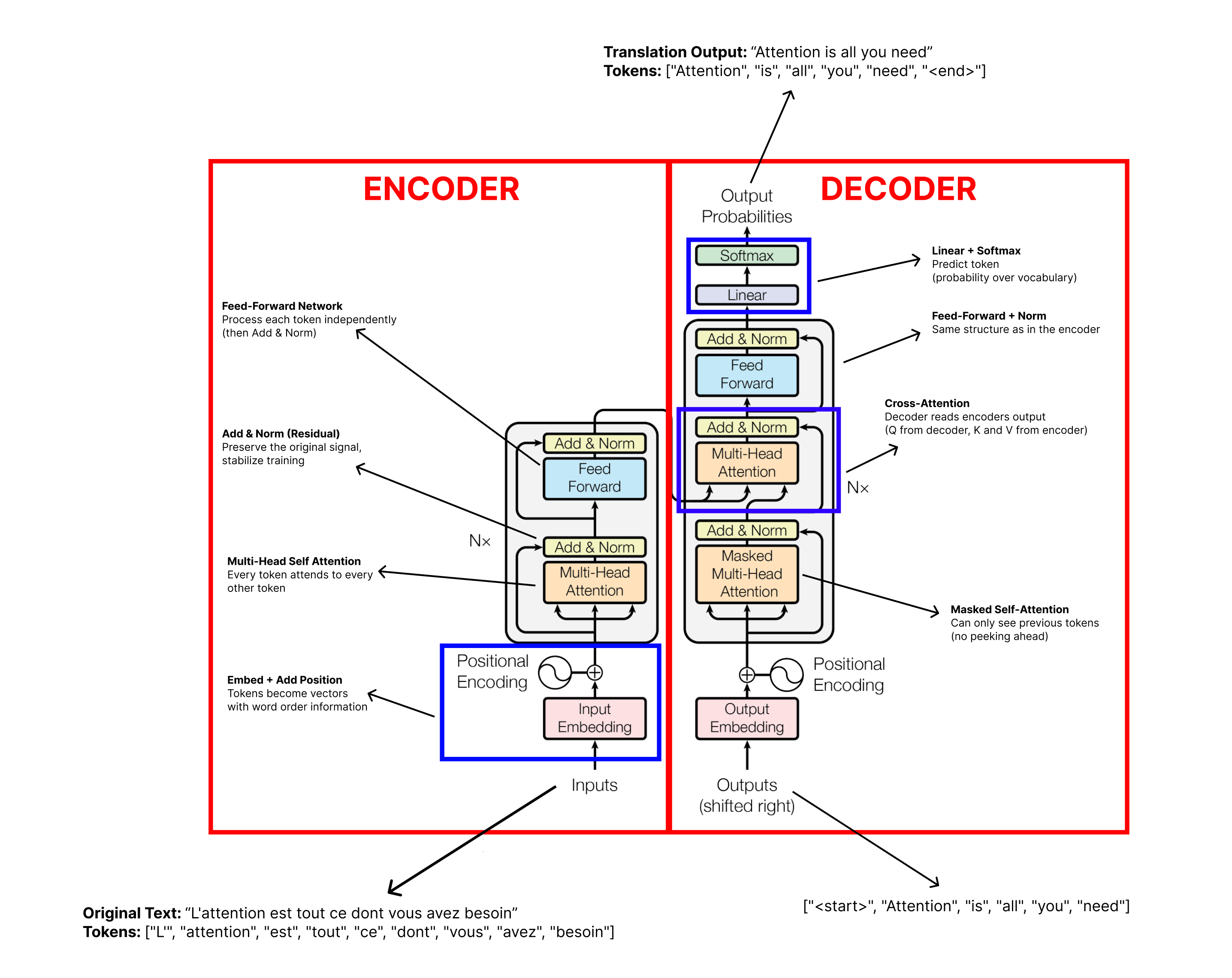
To summarize the data flow:
Input tokens get embedded and combined with positional encodings.
They pass through 6 encoder layers (self-attention + feed-forward, with residual connections and layer norm at each step).
The encoder’s final output is sent to the decoder.
The decoder takes the previously generated output tokens (also embedded with positional encodings), passes them through 6 decoder layers (masked self-attention + cross-attention + feed-forward).
The decoder’s output goes through a linear layer and softmax to produce the next token prediction.
That predicted token gets fed back in as input, and steps 4 and 5 repeat until the sequence is complete.
And that is the Transformer. Every component we covered in this section (attention, multi-head attention, positional encoding, feed-forward networks, residual connections, layer normalization) works together to create a model that can process entire sequences in parallel and learn complex relationships between tokens at any distance.
The original “Attention Is All You Need” paper tested this architecture on machine translation and achieved state-of-the-art results on both English-to-German and English-to-French benchmarks, while training significantly faster than the RNN-based models it replaced. The big Transformer model achieved a BLEU score of 28.4 on English-to-German (see Table 2), improving over the previous best by more than 2 points, after training for just 3.5 days on 8 GPUs.
But the real impact of the Transformer turned out to be far greater than that of machine translation. Researchers soon realized that parts of this architecture could be repurposed for a much more ambitious goal: building a general-purpose language model. That is where GPT comes in.
Act 3: From Transformer to GPT
The Big Bet: Decoder Only
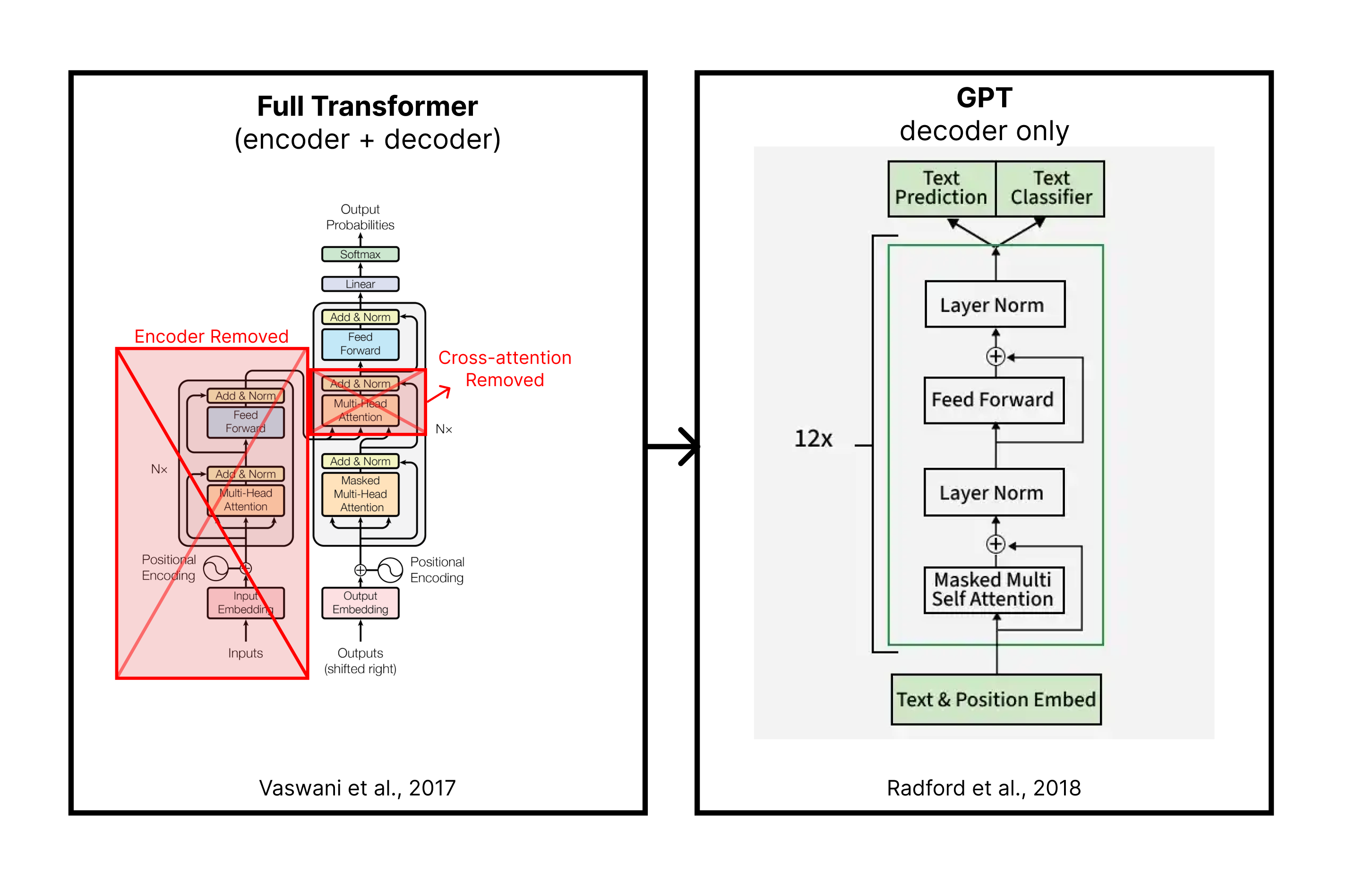
The Transformer we just walked through was designed for translation. The encoder reads a sentence in one language, and the decoder writes it in another. It is a sequence-to-sequence machine, and it was very good at that job.
But in 2018, researchers at OpenAI made a surprising and bold bet: what if you threw away the encoder entirely and just kept the decoder?
This bet gave birth to GPT (Generative Pre-trained Transformer). It doesn’t have an encoder, and there is no cross-attention, only a stack of decoder layers with masked self-attention, trained only to predict the next token.
It takes a sequence of tokens, and the model tries to predict the next token. Hence, the training objective is: given everything that came before, what is the most likely next token?
However, to predict the next word well, the model has to implicitly learn an enormous amount about language. It has to learn grammar (so sentences are well-formed), facts (so statements are plausible), reasoning patterns (so arguments follow logically), style and tone (so text sounds natural), and much more. All of these things are baked into the patterns of which words tend to follow which other words in real text.
The training process works like this:
Take a large chunk of text (from the internet, books, articles, code, etc.).
For each position in the text, the model sees all the tokens before that position and tries to predict the token at that position.
Compare the model’s prediction to the actual token. Compute a loss (how wrong was it?).
Use backpropagation to adjust the model’s weights slightly in the direction that would have made the prediction better.
Repeat this billions of times, across billions of tokens.
This is called autoregressive language modeling. “Autoregressive” just means each prediction depends on the previous ones. The model generates one token, feeds it back in as input, generates the next token, feeds that back in, and so on.
The architectural changes from the full Transformer are minimal:
No encoder. There is no separate “input understanding” module. The decoder is the whole model.
No cross-attention. Since there is no encoder, the cross-attention layer (where the decoder would read the encoder’s output) is removed. Each decoder layer now has just two sub-layers: masked self-attention and a feed-forward network.
Masked self-attention only. The model can never look at future tokens. When predicting token 5, it can only see tokens 1 through 4. This is the same masking we described in the decoder section, and it is essential for autoregressive generation.
That is the entire GPT architecture. The original GPT paper (Radford et al., 2018) used 12 decoder layers with a model dimension of 768, trained on BooksCorpus (roughly 7,000 books). It was solid proof of concept. What came next was much bigger.
How GPT Actually Generates Text
Understanding how GPT generates text is important because this is what is happening every time you use ChatGPT, Claude, Gemini, Grok, or any other AI chat tool. It all comes down to a loop.
Let’s walk through a concrete example. You type:
“The capital of France is”
Here is what happens:
Step 1. The model tokenizes your input: [“The”, “capital”, “of”, “France”, “is”]. Each token gets embedded, positional encodings are added, and the resulting vectors flow through all the decoder layers (masked self-attention, feed-forward, residual connections, layer norm, just like we covered).
Step 2. At the output, the model produces a probability distribution over its entire vocabulary (which could be 50,000+ tokens). Each token in the vocabulary gets a probability. “Paris” might get 0.92. “London” might get 0.03. “Berlin” might get 0.01. And so on.
Step 3. The model selects a token from this distribution. In the simplest case, it picks the one with the highest probability: “Paris.”
Step 4. That token gets appended to the input. Now the sequence is [“The”, “capital”, “of”, “France”, “is”, “Paris”]. The whole process conceptually repeats from Step 1 with this new, longer sequence (in practice, real systems use a technique called KV caching to reuse computations from previous steps and avoid redundant work). The model predicts the next token, maybe “.” or “,” and so on.
Step 5. This loop continues until the model produces a special end-of-sequence token, or until it hits a maximum length limit.
Here is a simplified version in code:
def generate(model, prompt_tokens, max_new_tokens):
    tokens = prompt_tokens
    for _ in range(max_new_tokens):
        probabilities = model(tokens)          # forward pass through all layers
        next_token = sample(probabilities)      # pick a token
        tokens = tokens + [next_token]          # append to sequence
        if next_token == END_OF_SEQUENCE:
            break
    return tokens
If you want to see a real (but still readable) implementation of this, Karpathy’s minGPT is about 300 lines of core code. It is a great way to see how simple the generation loop really is.
Temperature: Controlling Creativity
You might have noticed I said the model “selects a token from this distribution.” How it selects matters a lot, and this is controlled by a parameter called temperature.
Temperature = 0 (or very close to 0). The model always picks the single most likely token. This is deterministic so that you will get the same output every time for the same input. It tends to be more consistent, though not necessarily more correct, and can be repetitive.
Temperature = 1. The model samples proportionally to the probabilities. If “Paris” has a 0.92 probability and “Lyon” has a 0.02 probability, there is a small but real chance it picks “Lyon.” This adds variety and creativity, but it can also lead to incoherent or surprising outputs.
Temperature between 0 and 1. This is the sweet spot for most applications. The distribution is “sharpened” so high-probability tokens are even more favored, but there is still some randomness. Most AI tools you use operate somewhere in this range.
This is why you can ask ChatGPT the same question twice and get different answers. It is not “thinking differently” each time. The underlying probabilities remain the same, but random sampling selects different paths through the distribution.
Pre-training: Learning from the Internet
So, where does GPT get its knowledge? Pre-training is the process of training the model on a massive dataset of text before it is used for any specific task.
It’s an absurd amount of text. GPT-3, for example, was trained on roughly 300 billion tokens drawn from a mix of sources such as filtered web pages (Common Crawl), books, Wikipedia, and more. The model reads all of this text and learns to predict the next token, over and over, adjusting its weights with each example.
Through this process, the model picks up patterns at every level of language. It learns spelling and grammar (how words and sentences are typically formed). It learns facts (associations between entities and their properties, like “Paris is the capital of France”). It learns reasoning patterns (if A implies B and B implies C, then A implies C). It learns style and tone (how a legal document sounds different from a text message). All of this comes from the statistical regularities in the training data.
One important distinction, though, is that the model is not simply memorizing text. Most of what makes it useful is generalization, the ability to apply learned patterns to new inputs it has never seen before. When you ask it a question it has never encountered verbatim, it can still produce a reasonable answer because it has learned the patterns behind how questions like that tend to be answered. That said, models can and do memorize some sequences, especially ones that appear frequently in the training data. It is best to think of it as mostly pattern-learning with some memorization mixed in.
It is also worth briefly mentioning how the model sees text. As we covered in the building blocks section, models do not operate on whole words. They use subword tokenization schemes like Byte Pair Encoding (BPE) to break text into smaller pieces:
“unbelievable” might become [“un”, “believ”, “able”] (like we saw earlier)
“ChatGPT” might become something like [“Chat”, “G”, “PT”] (the exact split depends on the tokenizer)
This lets the model represent unfamiliar or rare words by composing them from smaller pieces it has seen before.
Here is what to keep in mind heading into Act 4:
Pre-training produces a general-purpose language model.
It can do many things (answer questions, write code, summarize text, translate languages), but it is not specifically optimized for any of them.
It is an incredibly capable autocomplete engine. However, you might ask it a question, and it might continue the text as if you were writing a webpage, generating more questions instead of an answer. Turning this raw capability into a helpful assistant requires additional training. That is where fine-tuning and RLHF come in.
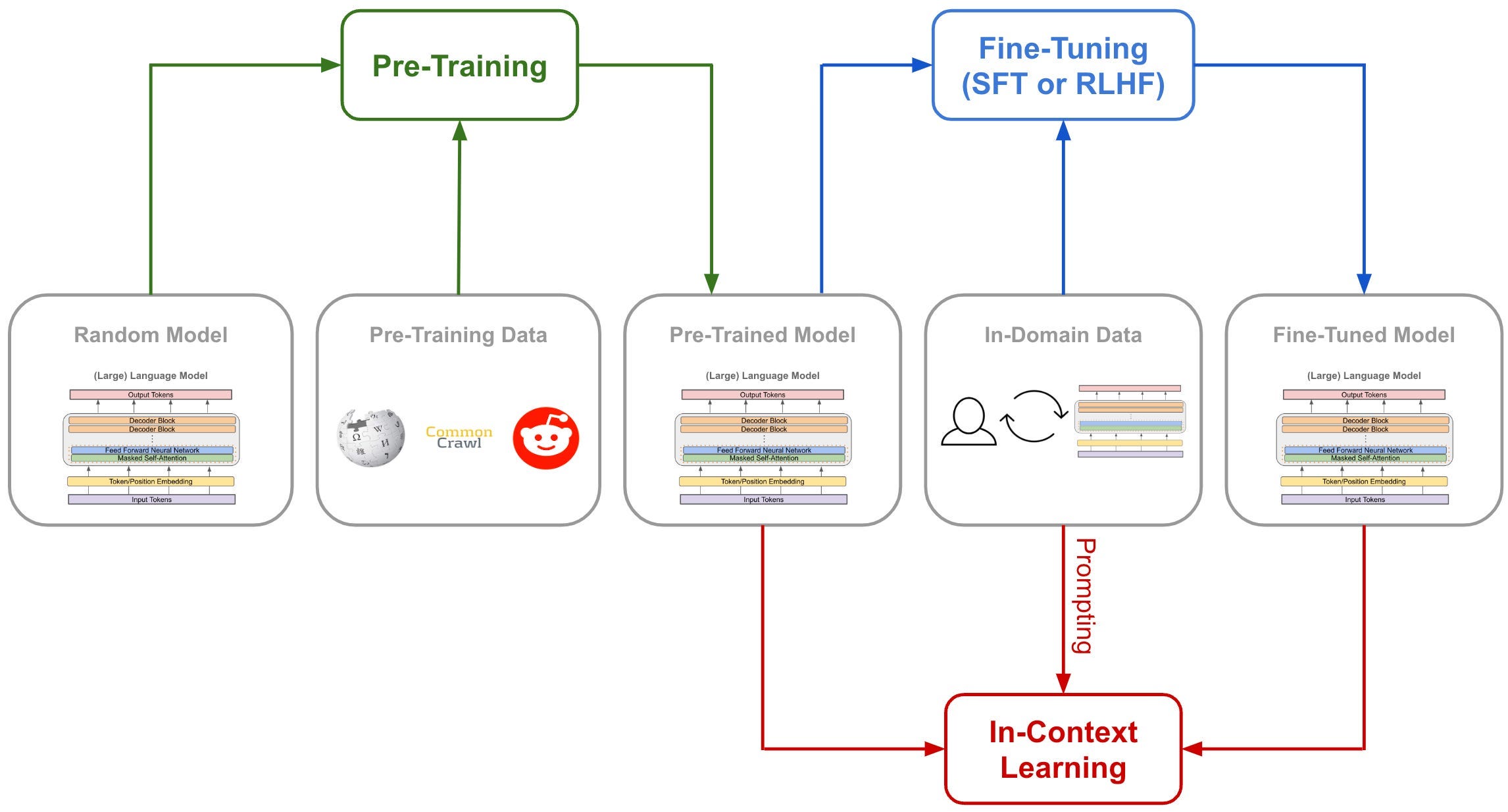
Image Source: Deep (Learning) Focus
Act 4: From GPT to LLMs
Scaling Laws: Bigger Is (Predictably) Better
GPT-1 started as a proof-of-concept. It showed that a decoder-only Transformer could learn useful language patterns simply by predicting the next word in a sentence. At 117 million parameters and 7,000 books’ worth of data, it was a solid achievement for 2018, even if it wasn’t a total game-changer yet.
What followed was a bit of a turning point for the industry: the discovery that AI performance improves predictably as you increase the model size, data, and training time.
This was formalized in a 2020 paper from OpenAI called “Scaling Laws for Neural Language Models” (Kaplan et al.). The key finding was that the model’s loss (how bad its predictions are) decreases as a power law along three axes:
Model size (number of parameters)
Dataset size (number of tokens trained on)
Compute (total amount of training computation)
What surprised people was how smooth and predictable this relationship is. You can plot model size on one axis and performance on the other, and it forms a clean curve. This means you can roughly forecast how good a model will be before you finish training it, just by knowing how big it is and how much data and compute you are throwing at it. It is not a guarantee, but it held up well enough to guide billions of dollars of investment.
The GPT family illustrates this scaling trajectory clearly:
ModelYearParametersNotable MilestoneGPT-12018117MProof of conceptGPT-220191.5BDeemed “too dangerous to release” at the timeGPT-32020175BFew-shot learning emergesGPT-42023UndisclosedMultimodal (text + images)
The important thing to notice is that there was no fundamental architectural change between GPT-1 and GPT-3. It is the same decoder-only Transformer, trained with the same next-token prediction objective. The difference is scale. More parameters, more data, more compute. And with that scale came capabilities that nobody explicitly programmed.
GPT-2 could generate surprisingly coherent paragraphs. GPT-3 could do things like answer questions, write code, and translate between languages, all without being specifically trained for those tasks. You could show it a few examples of a task (this is called few-shot learning), and it would figure out the pattern and apply it. This ability appeared as the model got bigger. It was not there in GPT-1, barely there in GPT-2, and clearly present in GPT-3.
But scale alone does not make a model helpful. A scaled-up GPT is still fundamentally an autocomplete engine. It predicts what text is likely to come next, not what text would be useful to a human. Getting from “impressive autocomplete” to “helpful assistant” required a different kind of training.
Fine-Tuning and RLHF: From Autocomplete to Assistant
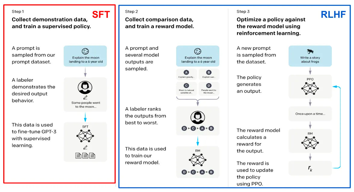
Image Source: Deep (Learning) Focus
Imagine you have a friend who has read the entire internet. They know an extraordinary amount about everything. But if you ask them a question, instead of answering it, they just continue your sentence as if they were writing the rest of a webpage. You ask “What is the capital of France?” and they respond with “What is the capital of Germany? What is the capital of Spain?” because on the internet, questions are often followed by more questions.
That is what a raw pre-trained GPT model is like. It has the knowledge, but it has not learned how to be helpful.
The fix comes in two stages.
Stage 1: Supervised Fine-Tuning (SFT)
The first stage is conceptually simple. You hire human annotators and have them write examples of ideal behavior. They write prompts (“Explain quantum computing to a 5-year-old”) and then write high-quality responses. You then train the model on these examples so it learns to imitate the style, format, and helpfulness of the human-written responses.
This is called Supervised Fine-Tuning (SFT). It uses the same training process as pre-training (predict the next token, compute the loss, backpropagate), but the training data is now curated conversations rather than raw internet text.
SFT gets you a long way there. After this stage, the model starts responding to questions with actual answers instead of continuing text. But it still has problems. It might give plausible-sounding but wrong responses. It might be unnecessarily verbose. It might produce outputs that are technically correct but not what the user actually wanted. These are subtle quality issues that are hard to capture with simple “predict the next token” training.
Stage 2: RLHF (Reinforcement Learning from Human Feedback)
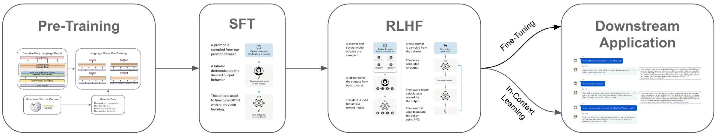
Image Source: Deep (Learning) Focus
This is the innovation that made ChatGPT feel different from everything before it.
The idea, introduced by OpenAI in their InstructGPT paper (Ouyang et al., 2022), is to train the model using human preferences rather than human-written examples. Here is how it works:
Generate multiple responses. For a given prompt, the model generates several different responses.
Humans rank them. Human raters look at the responses and rank them from best to worst. Which response is most helpful? Most accurate? Most safe? These rankings capture subtle quality differences that are hard to specify in a rule.
Train a reward model. Using those rankings, you train a separate model (called a reward model) to predict which responses humans would prefer. The reward model learns to assign higher scores to responses that humans rated highly.
Fine-tune with reinforcement learning. Finally, you use reinforcement learning (specifically an algorithm called PPO, or Proximal Policy Optimization) to adjust the language model so it generates responses that score highly with the reward model. The language model is essentially learning to produce outputs that humans would prefer.
In simple terms: SFT teaches the model what a good response looks like by showing examples. RLHF teaches the model why one response is better than another by learning from human preferences. Together, they turn a raw language model into something that feels like a helpful, conversational assistant.
This is a big part of why ChatGPT felt like such a step change when it launched in November 2022. The jump was not only about model size. A large part of the “ChatGPT feel” came from post-training with human feedback. OpenAI describes ChatGPT as a sibling model to InstructGPT, which was trained with RLHF to follow instructions. The model had been trained to care about what humans want, not just to predict the next word.
It is worth noting that RLHF is not the only approach. Anthropic (the company behind Claude) has developed related techniques called RLAIF (Reinforcement Learning from AI Feedback) and Constitutional AI, which supplement or replace human feedback in parts of the process. Meta and Google have also explored related alignment approaches. The details differ, but the core idea is the same: additional training after pre-training to make the model more helpful, harmless, and honest.
Reasoning: The “Thinking” Part
Remember the title of this post? “ChatGPT Doesn’t Think. It Pays Attention.” That is true in a fundamental sense. Everything under the hood is still attention and next-token prediction. But recent developments have pushed these models into territory that looks a lot like thinking, and it is worth understanding how.
Chain-of-Thought Prompting
In 2022, researchers at Google published a paper (Wei et al.) showing that if you prompt a language model to “think step by step,” its performance on complex reasoning tasks improves dramatically. This technique is called chain-of-thought (CoT) prompting.
For example, if you ask a model, “If a store has 3 apples and someone buys 2, then the store gets a delivery of 7 more, how many apples does the store have?” and just ask for the answer, it might get it wrong. But if you prompt it to work through the problem step by step, it performs much better because each intermediate step (3 - 2 = 1, then 1 + 7 = 8) becomes part of the generated text, and the model can attend to its own reasoning as it goes.
One way to think about this is that the model is doing its “reasoning” in the form of text it can read back. The intermediate steps are tokens, and the model attends to those tokens when generating the next ones. It is still next-token prediction, but applied to a reasoning trace that the model itself is producing. From this perspective, it is paying more attention rather than thinking in the way humans do.
Reasoning Models
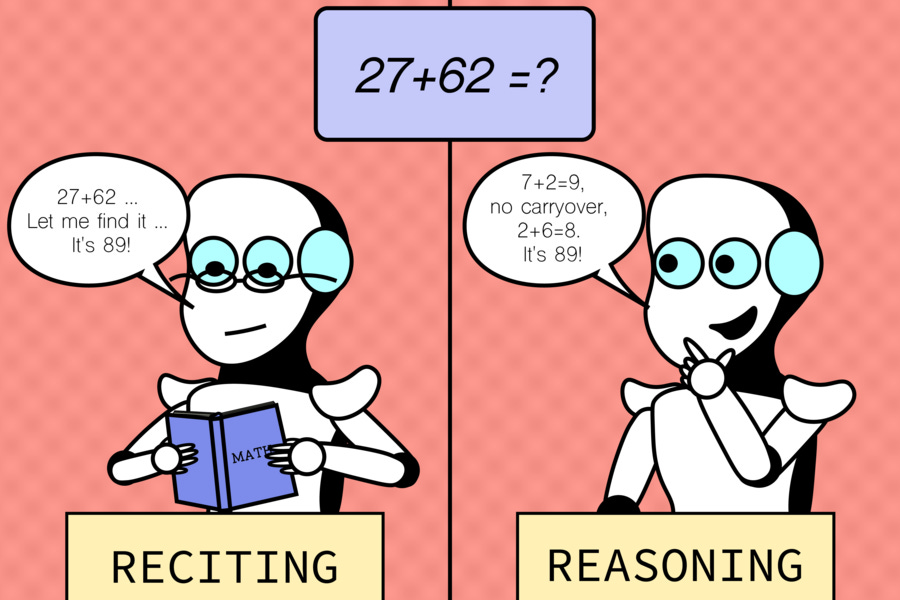
Image Source: MIT CSAIL
More recently, companies have taken this idea further by training models specifically to produce extended reasoning chains before giving a final answer. OpenAI’s o1 and o3 models and Anthropic’s Claude with extended thinking are examples.
These models are trained (often using reinforcement learning) to generate long internal reasoning traces. When you ask a complex question, the model might produce hundreds or thousands of tokens of step-by-step reasoning before arriving at an answer. The final answer tends to be significantly more accurate than what a model would produce if it tried to answer immediately.
The underlying mechanism is still attention and token prediction. But by training the model to produce intermediate reasoning steps, you effectively give it more “compute” at inference time. Instead of going directly from question to answer in a single pass, the model takes many steps, and each step can attend to all previous reasoning. It is similar to giving someone scratch paper for a math test versus asking them to do it all in their head.
So Does It Think?
This is one of the most debated questions in AI. The honest answer is it depends on what you mean by “think.”
If thinking means manipulating symbols step by step to arrive at a conclusion, then yes, reasoning models do something that looks like that. If thinking requires genuine understanding, consciousness, or intentionality, then no, these models are still doing sophisticated pattern matching over tokens.
What is clear is that these techniques produce better results on complex tasks. Whether you call it “thinking” or “structured token prediction” is partly a philosophical question. The practical reality is that the same core mechanism (attention + next-token prediction) can be steered to produce remarkably capable reasoning behavior through the right training and prompting techniques.
And that ties back to the title; even when the model “thinks,” it is paying attention.
Emergent Abilities and the LLM Paradigm
Something unexpected happened as language models got bigger. They started doing things that nobody explicitly trained them to do.
These are called emergent abilities (Wei et al., 2022), and they are one of the more surprising and interesting phenomena in modern AI. An emergent ability is a capability that is not present in smaller models but appears once the model reaches a certain scale. On some benchmarks, it can look like the ability turns on suddenly, almost like a phase transition, even though the underlying improvements may be more gradual than they first appear.
Examples include:
Few-shot learning. Show the model a few examples of a task it has never seen, and it figures out the pattern. GPT-3 could do this. GPT-2 mostly could not.
Chain-of-thought reasoning. The step-by-step reasoning we just discussed only works well in models above a certain size.
Code generation. Large models can write working code from natural language descriptions, even though they were trained primarily on text, not specifically on programming tasks.
Translation between languages the model saw relatively little of during training.
Arithmetic on numbers the model has never seen before (up to a point).
What makes this surprising is that none of these abilities were explicitly part of the training objective. The model was just trained to predict the next token. But at sufficient scale, next-token prediction apparently requires learning representations so rich that these capabilities come along for free.
This has led to a paradigm shift in how people think about AI systems. Before LLMs, the standard approach was to build a separate model for each task: one model for translation, one for summarization, one for question answering, and one for sentiment analysis. Each one required its own architecture, training data, and engineering effort.
The LLM paradigm is different. You train one very large model on a general objective (predict the next token), then adapt it to specific tasks through prompting, fine-tuning, or RLHF. This is why companies like OpenAI, Anthropic, Google, and Meta have invested so heavily in building larger and larger models. The returns from scale have been extraordinary so far.
Of course, whether this paradigm will continue to hold is an open question. There is active debate about whether emergent abilities are truly sudden or just artifacts of how we measure them. There are real limitations to what these models can do (they can still hallucinate confidently, struggle with certain types of reasoning, and make basic factual errors). And the cost of training and running these models is enormous, raising questions about sustainability and access.
But the trajectory from 2017 to today is remarkable. A single architecture, the Transformer, built on a single mechanism, attention, has gone from improving machine translation to powering the most capable AI systems ever built. And it all started with a paper titled “Attention Is All You Need.”
Act 5: Tying It All Together
We have covered a lot of ground. Let’s trace the full journey one more time.
It started with a problem. RNNs processed language one word at a time, struggling with long sequences and unable to take advantage of modern parallel hardware. Attention mechanisms helped, but they were bolted onto the sequential architecture rather than replacing it.
In 2017, a team of researchers at Google tried to find out what would happen if we dropped the sequential part and relied only on attention. The Transformer they built replaced recurrence entirely with self-attention, allowing every token to attend to every other token in a single step. With multi-head attention, they gave the model multiple perspectives on every word. And positional encodings preserved word order. On the other hand, residual connections and layer normalization kept training stable, and the final result was a model that could process entire sequences in parallel, learn long-range dependencies, and train significantly faster than anything before it.
Then came GPT, simplifying that architecture further. Researchers at OpenAI removed the encoder and cross-attention, relying only on the decoder stack, and trained it to predict the next token. The model also learned grammar, facts, reasoning, style, and more. Over time, we learned that as we scale up with more parameters and more data, we start to get capabilities that were never explicitly programmed. Finally, adding in fine-tuning and RLHF and we get a model that stops being a fancy autocomplete and starts acting like a helpful assistant.
Every time you talk to ChatGPT, Claude, Gemini, or any other AI assistant, this is what is happening under the hood. The input text gets turned into tokens, those tokens are embedded into vectors along with their positional information. Then they flow through layers of attention where every token attends to every other token, gathering context from across the entire input. Then the model predicts the next token. And the next. And the next. One token at a time, with each subsequent token informed by everything that came before.
It is attention, all the way down.
Writing this post over the past few weeks has been a big learning experience for me. The thing that surprised me most is how simple the core ideas are after I started to understand them. None of the individual components is complicated on its own; what makes them powerful is how they compose together and what happens when you scale them up.
I also came away with a deeper appreciation of the researchers behind this work. It is easy to look at the logic and think it is obvious, but it took years of work, building on decades of research in neural networks, sequence modeling, computing, and optimization, to arrive at something that looks this clean.
If you want to go deeper, attached below are resources that I found most valuable while learning the material. And if this is the first article you are reading in this series, be on the lookout for the other posts on AI agents and coding tools like Claude Code or Codex, building on the foundation laid here. Thanks for reading. I hope this helped demystify what is going on inside the AI tools you use every day. If you have questions, feedback, or corrections, I would love to hear from you.
ChatGPT doesn’t think. It pays attention. Now you know how.
Resources
Interactive Tools
Transformer Explainer (Georgia Tech Polo Club) - Interactive visualization where you can watch attention and data flow through a Transformer in real time. Spend an hour with this.
Karpathy’s minGPT - A full GPT implementation in about 300 lines of Python.
Karpathy’s nanoGPT - More recent and minimal GPT training repo. Pairs well with his YouTube walkthrough linked below.
Transformer Explainer source code - Source code for the Transformer Explainer tool.
Transformers in Action code - Code repository for the Transformers in Action book.
AnimatedLLM: Explaining LLMs with Interactive Visualizations, AnimatedLLM - Understanding the mechanics of LLMs (Includes text generation and training)
LLM Visualization - Interactive walkthrough of the internals of various LLMS such as nano-gpt, GPT-2, and GPT-3.
The Original Paper
“Attention Is All You Need” (Vaswani et al., 2017) - The paper that started it all. Worth reading even if you skip the math.
Video Explainers
3Blue1Brown: Large Language Models explained briefly - Short visual intro to LLMs, chatbots, pretraining, and tokens.
3Blue1Brown: But what is a GPT? Visual intro to Transformers - Visual explanation of how GPT works from the ground up.
3Blue1Brown: Attention in Transformers, visually explained - Step-by-step walkthrough of the attention mechanism.
3Blue1Brown: Visualizing Transformers and Attention (full talk) - Grant Sanderson’s full conference talk. More detailed than the shorter videos.
Andrej Karpathy: Let’s build GPT from scratch - Two hours of building a GPT from scratch in code. Long but worth it.
Andrej Karpathy: Deep Dive into LLMs like ChatGPT - General audience deep dive into LLM technology.
StatQuest: Transformer Neural Networks, Clearly Explained - Methodical, step-by-step walkthrough.
IBM Technology: How Large Language Models Work - Accessible overview from IBM.
Polo Club: Transformers Explained Visually - Video companion to the Transformer Explainer tool.
Umar Jamil: Attention is All You Need (including math) - Detailed walkthrough of the paper with math, inference, and training.
Leon Petrou: Transformers, explained - Another visual explanation of the architecture.
Further Reading
Jay Alammar: The Illustrated Transformer - Visual guide to the Transformer with diagrams for every component.
Sebastian Raschka: Understanding Self-Attention from Scratch - Code-first walkthrough of self-attention.
Lilian Weng: The Transformer Family Version 2.0 - Comprehensive survey of Transformer variants and improvements.
Lilian Weng: Attention? Attention! - Thorough overview of attention mechanisms from basics to advanced variants.
Christopher Olah: Understanding LSTMs - Classic post explaining LSTMs with diagrams. Good for understanding what came before Transformers.
Amirhossein Kazemnejad: Transformer Architecture - The Positional Encoding - Deep dive into positional encoding.
Transformers in Action (Nicole Koenigstein, Manning) - Hands-on book for implementing Transformers.
MIT 6.390: Introduction to Machine Learning - Transformers - Lecture notes on Transformers from MIT.
Google ML Crash Course: Introduction to LLMs - Google’s structured intro to large language models.
Hugging Face LLM Course: How do Transformers work? - Part of Hugging Face’s free LLM course.
Understanding AI: Large language models, explained with a minimum of math and jargon - Plain-language LLM explainer.
Miguel Grinberg: How LLMs Work, Explained Without Math - Another no-math explainer focused on intuition.
freeCodeCamp: A Beginner’s Guide to Large Language Models - Beginner-friendly intro.
IBM: What is a Transformer Model? - IBM’s overview of Transformers.
IBM: What are Large Language Models? - IBM’s LLM overview.
Stanford: AI Demystified - LLMs - Stanford’s introductory guide.
MIT News: Large language models use a surprisingly simple mechanism to retrieve stored knowledge - Research on how LLMs retrieve facts internally.
Key Papers
GPT-1: Improving Language Understanding by Generative Pre-Training (Radford et al., 2018)
GPT-2: Language Models are Unsupervised Multitask Learners (Radford et al., 2019)
GPT-3: Language Models are Few-Shot Learners (Brown et al., 2020)
GPT-4 Technical Report (OpenAI, 2023)
InstructGPT: Training language models to follow instructions with human feedback (Ouyang et al., 2022) - The RLHF paper behind ChatGPT.
Scaling Laws for Neural Language Models (Kaplan et al., 2020)
Chain-of-Thought Prompting Elicits Reasoning in Large Language Models (Wei et al., 2022)
Emergent Abilities of Large Language Models (Wei et al., 2022)
Constitutional AI: Harmlessness from AI Feedback (Bai et al., 2022) - Anthropic’s alignment approach.
Llama 2: Open Foundation and Fine-Tuned Chat Models (Touvron et al., 2023)
Neural Machine Translation by Jointly Learning to Align and Translate (Bahdanau et al., 2014) - The paper that introduced attention.
Sequence to Sequence Learning with Neural Networks (Sutskever et al., 2014) - The encoder-decoder paper.
Deep Residual Learning for Image Recognition (He et al., 2015) - Residual connections.
Layer Normalization (Ba et al., 2016)
RoFormer: Enhanced Transformer with Rotary Position Embedding (Su et al., 2021) - RoPE, used in many modern LLMs.
Efficient Transformers: A Survey (Tay et al., 2020)
FlashAttention: Fast and Memory-Efficient Exact Attention (Dao et al., 2022)
Transformer Explainer: Interactive Learning of Text-Generative Models (Cho et al., 2024)
Are Emergent Abilities of Large Language Models a Mirage? (Schaeffer et al., 2023)
Thank you for demystifying this alien stuff for mere mortals like me. A long read, though, but I will get through it. The more I read, the more of an eye-opener it is to the mysterious world of AI. Keep up the good job on the “notebook”. GOD Bless Abundantly.